Numerical integration

We could write our own function to do just that. In R, a bare-bones implementation of numerical integration would look something like this:

integrate_numerically <- function(f, a, b, n = 20) {
  dx <- (b - a) / n
  x <- seq(a, b - dx, dx)
  sum(f(x) * dx)
}

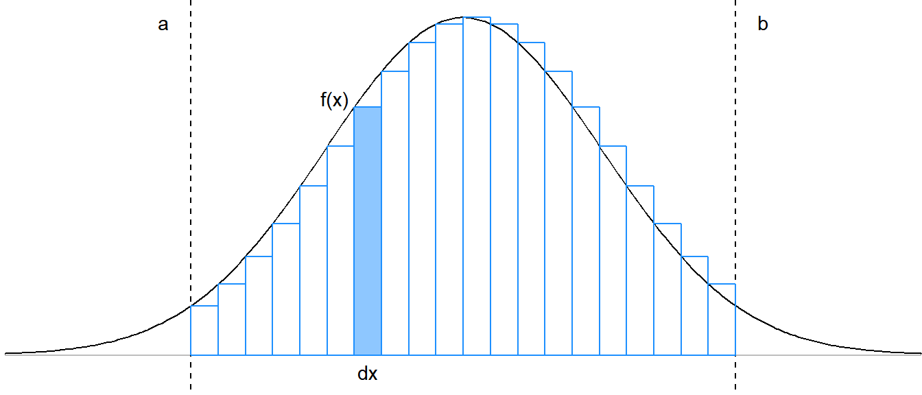
This function finds the area under a curve \(f\), between points \(a\) and \(b\), by splitting the interval \([a,b]\) into \(n\) smaller “sub-intervals”, and then approximating the area in each sub-interval with the area of a rectangle.

For each sub-interval, the approximating rectangle has width equal to the width of the sub-interval, or “\(dx\)”, and height equal to the value of the function \(f\) evaluated at the starting point of the sub-interval.

Here’s a quick diagram³ to illustrate:

integrate_numerically(dnorm, -1.96, 1.96)

## [1] 0.9492712

Fortunately we don’t have to be content with that. Since numerical integration is an important computational tool that comes up in many applications, smarter people already thought about it more carefully, and implemented the integrate function. (It does numerical integration too, but better.) Our implementation isn’t awful for this specific problem, but it could be a lot more efficient.

integrate(dnorm, -1.96, 1.96)

## 0.9500042 with absolute error < 1e-11

Expected values with numerical integration

Well, we eventually made it here! The point that we’ve been slowly approaching here is: that based on the formulae presented earlier in the maths bit, we can use integrate to find the expected value of a random variable, or a transformation of one, given its PDF. Here’s how:

integrate(function(x) x * dnorm(x, mean = 5), -Inf, Inf)

## 5 with absolute error < 6e-05

We could wrap this in a function for finding the mean:

find_mean <- function(f, ..., from = -Inf, to = Inf) {
  integrate(function(x) x * f(x, ...), from, to)
}

And then try it out with some simple distributions:

find_mean(dexp, rate = 2)

## 0.5 with absolute error < 8.6e-06

But it could also be useful to generalise a bit, and create a function factory instead. That would be a good way to avoid duplicating code if we wanted to find other moments, or indeed expected values of transformations. The idea is to make a function that, given a transformation function, will return another function that finds the expected value of that transformation of a random variable:

ev_finder <- function(transform = identity) {
  function(f, ..., from = -Inf, to = Inf) {
    integrate(function(x) transform(x) * f(x, ...), from, to)
  }
}

Since we know that finding moments of PDFs can be seen as a special case of expected values of transformations, we can wrap ev_finder here to define another function factory, this time for easy generation of functions to find moments.

moment_finder <- function(n, c = 0) {
  ev_finder(function(x) (x - c) ^ n)
}

Then, using moment_finder, we could define find_mean from before with one line. But moment_finder also makes it simple to define a function to find the variance (i.e. the second central moment):

find_mean <- moment_finder(1)
find_variance <- function(f, ...) {
  mu <- find_mean(f, ...)$value
  moment_finder(2, mu)(f, ...)
}

And again, we can try it out on some distributions:

find_variance(dnorm, mean = 2, sd = 2)

## 4 with absolute error < 2.5e-06

find_variance(dexp, rate = 1 / 4)

## 16 with absolute error < 0.00051

There we go! Expected values for random variables and transformations – sorted.